If you're running an A/B test using standard statistical tests and look at your results early, you are not getting the statistical guarantees that you think you are. In How Not To Run An A/B Test, Evan Miller explains the issue, and recommends the standard technique of deciding on a sample size in advance, then only looking at your statistics once. Never before, and never again. Because on that one look you've used up all of your willingness to be wrong.
This suggestion is statistically valid. However it is hazardous to your prospects for continued employment. No boss is going to want to hear that there will be no peeking at your statistics. But suppose that you have managed to get your boss to do that. Then this happens:
"So how is that test going," your boss asks.
"Well," you say, "we reached 20,000 visitors this morning, so I stopped the test and have the results in front of me."
"Great!" your boss exclaims, Which version won?"
You grimace, "Neither. The green button did a bit better, but we only had a p-value of 0.18, so we can't draw a real conclusion at the 95-percent confidence level."
Your boss looks confused, "Well, why did you stop it? I need an answer. Throw another 20,000 visitors at it."
"Well," you say slowly, "we can't. We've used up our allowed five percent of mistakes. We can't just collect more data, we have to accept that the experiment is over and we didn't get an answer. Hopefully we're more lucky with our next A/B test."
They call this a "career limiting conversation." Even if you somehow convince your boss that the math is right, people will wonder why nobody else seems to have this pain point The online testing tools don't discuss it. Blog articles don't mention it. Eventually you'll get replaced by someone who has never heard of Evan Miller. The stats will get done incorrectly. The business will get the answers they want to hear. And nobody will care that you were right.
The good news is that you can be right, without putting your job at risk. This article will explain one valid approach which lets you look at the statistics as often as you like, run tests as long as you need to, and still gives you good guarantees that you will make very few chance errors. This is not the only reasonable approach to use. Future articles will explore others, and discuss the trade-offs that could lead you to prefer one over the others.
The upside of doing math right is that we can believe our results. The downside is that we have to do math. We'll limit that math to adding, subtracting, multiplying, dividing, square roots, basic algebra, running computer programs and looking at pretty pictures. But first we need to understand how things are set up so that the rest of it makes sense.
To start with we have a website. Visitors come, and are assigned one of two experiences, A or B. Once you've been assigned an experience, we will make sure that you consistently get that. Some of those users will go through some conversion event, such as signup. For each visitor we will track the first time they go through that conversion event (if ever) and record that fact then. Note that we do not track people who are in the test - just the actual sequence of conversions. This data collection procedure likely is different than what you've seen before, but it will prove sufficient.
So we record a sequence of conversions. Let us suppose that, on average, $r_A$ is the fraction of the people who will convert if they are put into version A. Similarly the average conversion rate for version B is $r_B$. We do not know exactly what those conversion rates are, nor are we going to try to figure that out. All we want to know is which one is bigger, so that we know which one we want everyone to get.
After a very large number of people convert, what portion of them should be A? Well if we have $v$ visitors, then on average $\frac{v}{2}$ wound up in each version. Then:
$$\begin{eqnarray} \text{Portion that are A} & = & \text{# of A's} / \text{# of conversions} \\ & = & \text{# of A's} / (\text{# of A's} + \text{# of B's}) \\ & = & (\frac{v}{2} r_A) / (\frac{v}{2} r_A + \frac{v}{2} r_B) \\ & = & r_A / (r_A + r_B) \\ & = & \frac{r_A}{r_A + r_B} \frac{1/r_A}{1/r_A} \\ & = & \frac{1}{1 + \frac{r_B}{r_A}} \end{eqnarray}$$
If then less than half of the conversions will be in A. But if then more than half of the conversions will be in A. Therefore the ratio $\frac{r_B}{r_A}$ tells us which version is better.
What else do we know about this sequence? Well, if conversion is assumed to be instantaneous, we can make the incredibly strong claim that the sequence of A's and B's that we get behaves statistically like a series of independent (but likely biased) coin flips. At first this seems like an amazing claim - after all every time we we get an A, that is evidence that we put a visitor into A who could have gone into B instead - isn't there correlation of some sort there? But the following thought exercise shows why it is true. First let's randomly label all possible visitors, whether or not we ever see them during the test, A or B. Then as they arrive, instead of labeling them, we just observe the label they already have. It is now clear that what happens with the A's is entirely independent of what happens with the B's.
But there is no statistical difference between what happens if we label everyone randomly in advance, then discover those labels as they arrive, versus randomly labeling visitors as they arrive. Therefore in our original setup what we observe looks like independent flips of a biased coin.
The mathematically inclined reader may wish to insert verbiage about Poisson processes, and demonstrate that this conclusion continues to hold if the actual conversion rates vary over time and conversion is not instantaneous - just so long as the ratio of rates remains constant, and the time to convert for conversions has the same distribution of times. (You can actually relax assumptions even more than that, but that generality is more than we need.)
In the last section we found that the sequence of conversions statistically looks like a sequence of independent coin flips with A coming up with a fixed probability. Therefore we're faced with a series of decisions. At each number of conversions $n$, we have $m$ more A conversions than B conversions ($m$ can, of course, be negative). Given $n$ and $m$, we have to decide whether to declare the test done, or say that we do not know the answer and should continue the test.
There are a variety of ways to analyze this problem. We will follow Evan's lead and use a frequentist approach. Which means that we will construct a procedure which, if there is no difference, be unlikely to incorrectly conclude that there is bias. Of course if there is bias, we will be even less likely to make the mistake of calling the bias backwards, so the hypothesis that the versions convert equally is our worst case.
We wind up with something similar to Evan's approach if we wait until we reach a pre-agreed number of conversions, and then try to make up our minds based on the data we now have. This leads to the following problems that our hypothetical boss was rightly unhappy about before:
Our trick is to always be making decisions, but at a carefully limited rate so that the cumulative likelihood of wrongly deciding that there is a bias when there isn't remains bounded. To that end let us define our maximum cumulative decision limit to be the function $\frac{p n}{n + 10000}$ where $1 - p$ is the desired confidence level that we want to make decisions of. There is nothing special about this function other than the fact that it starts at $0$, gets close to $p$ as $n$ gets large, and happens to be fairly easy to write down. In fact it is just a complicated analog of setting the target sample size at which you plan to compute statistics with Evan's procedure.
Given this function, here is how we can generate our procedure. We can write a computer program that estimates the distribution of $m$ (the difference between how many were A and B) for each number of conversions $n$. For any $n$ where we find that we can decide to stop the test for the most extreme value of $m$ without having our cumulative probability of making a decision exceed the limit function above, we do. This generates a sequence of potential stopping points where we could stop the test. Then when we're running an A/B test, we can at any point look at the number of conversions, and the difference between how many are A and B, then compare with the output of that program and decide whether or not to stop.
This computer program is not hypothetical, and was not that hard to write. Here is the start of an actual sample run.
 bin/conversion-simulation --header --p-limit 0.05 | head
 conversions    difference  finished    standard deviations p-value
 15 15  6.103515625e-05 3.87298334620742    0.000107512
 20 18  8.96453857421875e-05    4.02492235949962    5.6994e-05
 24 20  0.000111103057861328    4.08248290463863    4.4558e-05
 28 22  0.000124886631965637    4.1576092031015 3.216e-05
 31 23  0.000141501426696777    4.13092194661582    3.6132e-05
 34 24  0.000158817390911281    4.11596604342021    3.8556e-05
 37 25  0.000175689201569185    4.10997468263393    3.957e-05
 40 26  0.000191462566363043    4.11096095821889    3.9402e-05
 43 27  0.000205799091418157    4.11746139898033    3.8306e-05
This is outputting a tab delimited file describing a $95\%$ confidence procedure. The columns of interest are conversions and difference. So, for instance, when we get to 15 conversions, if all 15 are of the same type, we can stop the test. If we get to 20 conversions and all but one are of the same type, we can stop the test. And so on.
Making a decision on every single conversion is the possible worst case for making repeated significance errors. Unless you automate your tests, Odds are that you will look less often and make fewer errors. But, as Evan notes, it is during your first few looks that you will experience the majority of your repeated significance errors. Therefore it is reasonable to use the thresholds for this procedure, even if you do look less often.
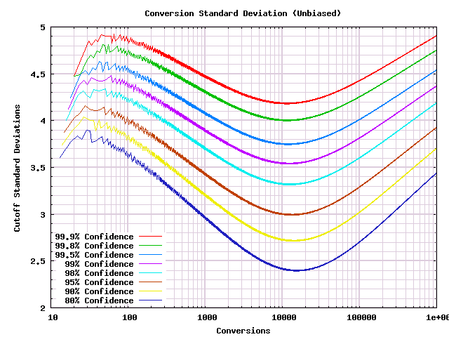
That program creates a lot of output, that is easier to understand in a graph. I picked a variety of target confidence levels from $80\%$ (more errors than most want to accept) to $99.9\%$ (for organizations who run lots of tests and want them all to be right. I ran each to a million conversions, and then plotted them on the following graph.
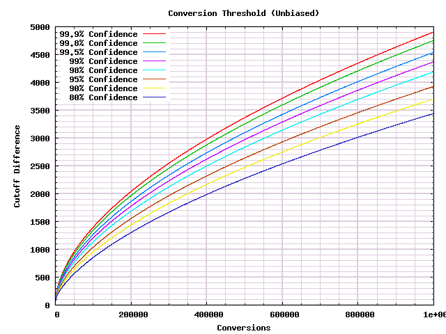
In this form the graph is hard to use because the exact cutoff numbers are hard to make out, particularly for small sample sizes. But if you've got statistics experience, the first thing you'll naturally notice is that the shape looks similar to the square root of the number of conversions. In statistics, data often spreads out like a square root, so it is worth trying to divide by the square root to see if we get a more useable graph.
(This paragraph is for people who have taken probability theory or statistics. Please skip if you don't remember that material.) You may remember that the sum of a series of random variables looks like a normal distribution with mean the sum of the means and variance the sum of the variances. That distribution spreads out according to the standard deviation which is the square root of the variance. In our case our random variables are coin flips with value +-1. Under the null hypothesis the mean is 0, the variance is 1, so the distribution after $n$ conversions is a normal with mean 0 and standard deviation $\sqrt{n}$. Therefore we should expect that everything should scale according to the standard deviation, and dividing by it will normalize the graph in a more useful way.
This graph is somewhat complicated, but it lets us calculate A/B test results by hand. I will illustrate the method with numbers that came up in a test that ZipRecruiter was running while I was writing this section. In that test there were $316$ A conversions, and $417$ B conversions.
But this graph tells us more. It can give us a decent idea how much more data we need to use this procedure than we may have been used to using. For instance let's look at the $95\%$ confidence curve. In the graph that curve is mostly between $3$ and $4$ standard deviations. But if you look on a standard table of normal distributions, a $95\%$ confidence threshold is about $2$ standard deviations out. (Actually $1.96$.) Therefore we need to get to $1.5$ to $2$ times as many standard deviations under this procedure. If you have a persistent bias, after $x^2$ times as much data has been collected, a standard deviation is $x$ times as big, and your bias has added up to $x$ times as many standard deviations. Therefore, as a back of the envelope, you're going to need $2.25$ to $4$ times as much data to reach $95\%$ significance under this test than you would if you were being less careful. Of course the upside is that you get valid statistics without having to guess in advance how much data you will need.
For our next trick, let's convert that graph to show the kinds of p-values that we're used to seeing from more traditional statistical tests. Remember that small p-values are many standard deviations out, so the order of the curves flips. Also I will use a log-log scale so that the data is readable.
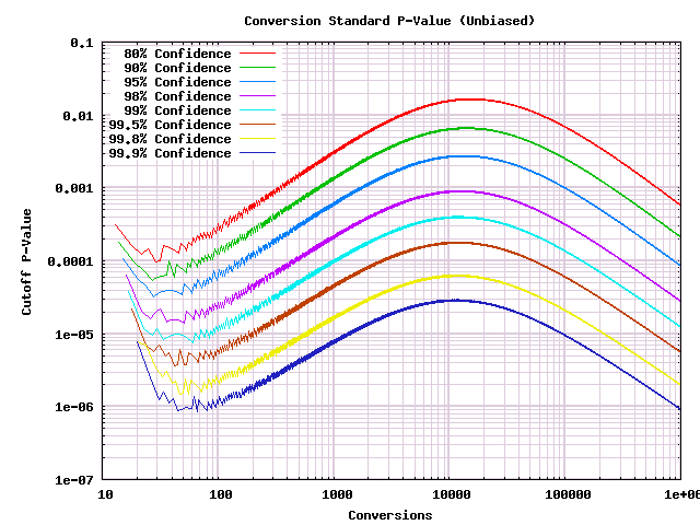
This graph tells us two things. First of all, if you've got p-values that are being reported using any of a variety of frequentist statistical tests, this can be used to derive rules on whether to stop the A/B test. Secondly if you have been doing multiple looks in the past, this gives you an idea of what level of confidence you've actually been deciding things at. (As Evan claims, it is probably much worse than you thought it was!)
OK, so that is how you use these graphs, but why does it have that shape? In one sense it doesn't really matter, since the details have to do with the arbitrary cutoff rule that we used. But understanding the shape is a good sanity check that we have not gone far astray. Feel free to skip this if you're not interested.
This article has walked through a very different way of of solving the issue of repeated significance testing errors that Evan Miller raised in How Not To Run An A/B Test. The big advantage of this procedure over the standard statistical approach that Evan Miller recommends is that you will find yourself able to stop bad tests fast, and keep running slow tests until they eventually reach significance. This avoids painful conversations that are likely to leave various co-workers (including your boss) frustrated with you.
This article described a universal procedure that hits a very strong statistical standard. See this picture for how you can evaluate it by hand. Following this standard requires several times more data than you would use if you were less careful (or if you avoided multiple looks). In practice this procedure is better than is actually needed, but that will be a topic for another article.
My thanks in chronological order to Benjamin Yu, Kaitlyn Parkhurst, Curtis Poe, Eric Hammond, Joe Edmonds, Amy Price, and one more who asked to be anonymous for feedback on various drafts. Without their help, this article would have been much worse. Any remaining mistakes should be emailed to Ben Tilly.
Further discussion of this article may be found on Hacker News.